|
|
Misop tutorial MiSeq 2x250 PE reads, mouse feces and mock community samples |
Part 1: UPARSE pipeline (reads to OTU table)
Part 2: Mock community analysis (stringent)
Part 3: Mock community analysis (less stringent)
Part 4: Read quality and error rate analysis
Part 4. Mock community read quality and error rate analysis
The usearch_global command has a feature which performs detailed analysis of mock community reads by comparing them with a reference database for the community. The -qout option specifies the name of a report file. Example command lines are found in the run_mock.bash and run_mock1.bash scripts:
$usearch -usearch_global $out/merged_nonch.fq -db ../ref/HMP_MOCK.v35.fasta \
-strand plus -qout $out/qout.txt -log $out/qout.log -id 0.9
You can find the qout.txt and qout_filtered.txt files in the out/mock and out/mock1 subdirectories, or follow this link to see a typical report.
If a read does not match a reference sequence exactly, then differences are considered to be errors. You should use chimera-filtered reads to get the best estimate of Q score accuracy and the overall error rate. The identity threshold of 0.9 is designed to capture most reads with errors while filtering out most contaminants, though as we saw in Part 2 of this tutorial there is a low-frequency contaminant with 94% identity so this won't work perfectly. You could increase the threshold to 0.95, but then you might miss some of the worst reads.
The report starts with a summary of the substitution and indel rates:
35 Reads with > 3% errors (0.745%)
0.151% Mean subst. error rate (1772 errs, 1174911 bases)
0.000% Mean insert error rate (0 errs, 1174911 bases)
0.002% Mean delete error rate (20 errs, 1174911 bases)
This shows that we have a very low average rate of 0.2% base call errors. However, we have 35 reads with >3% errors, which will create up to 35 spurious OTUs. The file qout_filtered.txt has the results after quality filtering by maximum expected errors at a threshold of 1.0:
5 Reads with > 3% errors (0.113%)
0.080% Mean subst. error rate (887 errs, 1109427 bases)
0.000% Mean insert error rate (0 errs, 1109427 bases)
0.002% Mean delete error rate (18 errs, 1109427 bases)
Notice that we kept 1109427/1174911 = 94% of the data and fitered 30/35 = 86% of the reads with >3% errors. Most of the 6% reads that were discarded by the filter map back to OTUs, so the cost in sensitivity is negligible compared with the improvement in spurious OTUs.
Next is an analysis of the Q score accuracy.

For each Q score in the FASTQ files, the number of bases and number of diffs (errors) is reported. Pex is the error probability predicted by the Phred score and Pobs is the observed probability, calculated as the number of differences divided by the number of bases. This gives the observed quality score, calculated as Qobs = –10 log10(Pobs). In the above example, you can see that Q=3 and Q=4 both are pretty good: the observed error rate gives Q=4 in both cases, not bad for a small sample and considering how difficult it is to estimate an error probability.
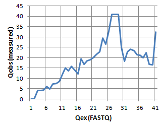
Following this human-readable table is a section starting with "Q to Qobs tabbed" which gives Q and Qobs in tabbed-text format, read to be copy-pasted into a program for charting, e.g. Excel. Using the unfiltered data from qout.txt, the plot looks like this:

We see good agreement up to around Q=25, then we see that the measured Q scores are lower than the Q scores in the FASTQ file, which means that the Q scores are over-optimistic (we get more errors than predicted). This is not necessarily because the machine Q scores have low accuracy or the merged Q scores are overestimated -- notice from the table that the frequencies of these Q score values is very low (0.01% to 0.1%), and PCR errors will cause Qobs to be systematically underestimated, we just don't know by how much.
The EE table shows how well expected errors predicts the observed number of differences:

EE is the integer-rounded number of expected errors, N is the number of reads, N is the total number of differences observed in those reads, Div is the divergence (mean % difference between the read and the closest reference sequence) and AvgE is the mean number of observed errors (differences). In this example we see that EE predicts the number of errors very well: AvgE is close to E, which justifies the use of an expected error quality filter.
The Poisson table shows a least-squares fit to a Poisson distribution.

If base call errors are independently and identically distributed (IID), then the number of errors should be Poisson distributed. If errors correlate in bad reads, then we would expect a "fat tail", i.e. more reads with high error rates than the Poisson distribution predicts. This is exactly what we see in the above table, for example we see 0.3% reads with 5 errors while the Poisson distribution predicts 0.001%. Again, it is not clear whether this is due to PCR errors or true correlations between bad bases. My guess is that there is a contribution due to correlation and the tail really is fat, but this is difficult to check empirically with amplicon sequencing because PCR errors cannot be reliably distinguished from sequencer error. With shotgun sequencing it is easy to check, but we can't assume the results apply to amplicon sequencing with Illumina because the basecaller analysis is more difficult when there are many similar clusters in the image.